Duplicate data can sometimes be useful, but it often complicates data analysis. It’s better to find, highlight, and review duplicates before removal rather than deleting them immediately.
To remove duplicates, first select the range of cells containing the duplicate values you want to remove. Ensure that any outlines or subtotals are removed from your data beforehand.
Go to Data > Remove Duplicates, and then check or uncheck the columns you want to clean up before clicking OK.
Excel provides a built-in tool to delete duplicate entries. Follow these steps to remove duplicates in Excel:
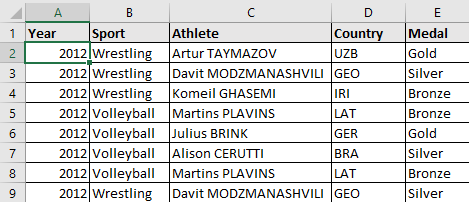
Step 1: Click on any cell or a specific range within the dataset from which you want to remove duplicates. If you select a single cell, Excel will automatically determine the range for the next step.
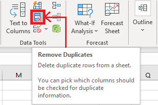
- Step 2: Next, locate the ‘Remove Duplicates’ option and select it. DATA tab → Data Tools section → Remove Duplicates
-
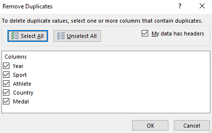
Step 3: A dialog box will appear, allowing you to select the columns you want to compare for duplicate data.
If your data includes column headers, check the ‘My data has headers’ option, and then click OK.
By selecting the header option, the first row will be excluded from the duplicate removal process.
-
Step 4: Excel will then delete the duplicate rows and display a dialog box summarizing the process. The dialog box will show the number of duplicate values found and removed, along with the count of unique values that remain.
Step 5: You will see that the duplicate records have been successfully removed.
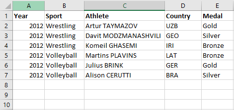
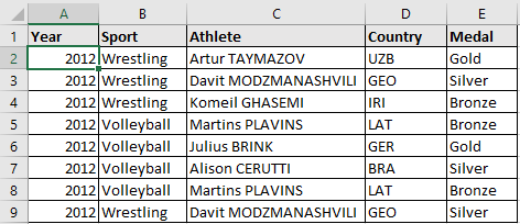
Let’s explore how to remove duplicates in Excel using the Advanced Filter option.
Understanding Filtering for Unique Values vs. Removing Duplicate Values
When you aim to create a list of unique values, you can either filter for unique values or remove duplicate values. Both tasks serve a similar purpose, but there’s a key difference. Filtering for unique values hides the duplicate entries temporarily, while removing duplicate values deletes them permanently.
It’s also important to note that the comparison of duplicate values is based on what is visible in the cell, not the underlying value. For example, if two cells contain the same date but are formatted differently, such as “3/9/2022” and “Mar 9, 2022,” Excel treats them as unique values.
Therefore, it’s a good practice to filter or conditionally format unique values first to ensure you get the expected results before removing duplicates.
Filtering for Unique Values
Follow these steps to filter for unique values:
- Select the Range of Cells: Start by selecting the range of cells. Ensure that the active cell is within a table.
- Locate the Advanced Filter Option: Go to the Data tab, then find and select the Advanced filter option in the Sort & Filter group.
- Path: Data tab → Sort & Filter section → Advanced.
- Advanced Filter Popup Box:
- If you want to filter the range of cells or table in place, select the “Filter the list in place” option.
- If you want to copy the results of the filter to a different location, follow these steps:
- Select “Copy to another location.”
- In the “Copy to” box, enter the cell reference where you want the unique values to be copied.
- You can temporarily click the “Collapse Dialog” button (🡓) to hide the popup window. After selecting the target cell, click the “Expand” button (🡑).
- Check the “Unique records only” option box, then click OK.
Using the Advanced Filter Option
The Advanced Filter option in Excel allows you to filter out duplicate values and copy the unique ones to a different location. Here’s how to use it:
- Select a Cell or Range: Click on a cell or a range within the dataset where you want to remove duplicates. If you select a single cell, Excel will automatically determine the range when you click on Advanced Filter.
- Proceed with the Advanced Filter: Follow the steps outlined above to filter for unique values or copy them to a different location.
This method is particularly useful when you want to keep the original dataset intact and work with a filtered list of unique values elsewhere.
Become The Highest-Paid Business Analysis Expert
With Business Analyst Master’s ProgramExplore Now
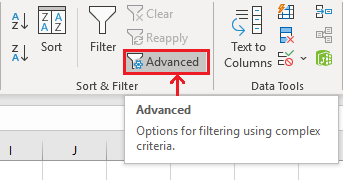
- Locate the Advanced Filter option.
DATA tab → Sort & Filter section → Advanced and click on it.
-
You will see a dialog box that provides a list of options for advanced filtering.
- Select ‘Copy to Another Location’: Choose this option if you want to copy the unique values to a different location within your worksheet.
- Verify the ‘List Range’: Ensure that the range of your records in the ‘List Range’ field matches the range you specified earlier.
- Specify the ‘Copy to’ Location: In the ‘Copy to:’ field, enter the range where you want the unique values to be copied.
- Check ‘Unique Records Only’: This is the most crucial step—make sure to check the ‘Unique records only’ box to filter out duplicates.
- Click OK: After confirming your selections, click OK to execute the filter and copy the unique values to the specified location.
- The unique values will be copied to cell G1.

Now that we’ve covered the in-built functionalities in Excel for removing duplicates, let’s move on to creating our own function to achieve the same.
How to Use Formulas to Remove Duplicates in Excel
We’ll demonstrate this approach using a simple example with columns for the type of sport, athlete name, and medal won.
Step 1: Set Up Your Data
Start by organizing your data into columns. For this example, we’ll use:
- Column A: Type of Sport
- Column B: Athlete Name
- Column C: Medal Won
Step 2: Create a Helper Column
To identify duplicates, we will create a helper column that flags them.
- In Column D (Helper Column), enter the following formula in the first row and drag it down to apply it to all rows:
excel
=IF(COUNTIF($A$2:A2,A2&B2&C2)>1,"Duplicate","Unique")
This formula checks if the combination of the sport, athlete name, and medal has already appeared in the rows above. If it has, it marks the entry as “Duplicate”; otherwise, it marks it as “Unique.”
Step 3: Filter or Remove Duplicates
- Filter for Unique Values: You can now filter the Helper Column to show only “Unique” values, leaving out the duplicates.
- Remove Duplicates: If you want to remove duplicates, you can delete the rows marked as “Duplicate” in the Helper Column.
This method is useful when you need more control over how duplicates are identified, especially when they are determined by combinations of multiple columns rather than individual values.

This method involves combining the columns using an Excel formula to identify duplicates based on the combined data. We’ll then filter out the duplicate values—those that appear more than once.
Step-by-Step Process:
- Combine Columns:
- To identify duplicates, you first need to combine the values in columns A, B, and C.
- In cell D2, enter the following formula to concatenate the values:
excel
=A2&B2&C2
- This formula merges the values from columns A, B, and C into a single string in column D.
- Copy the Formula:
- Drag the formula down from cell D2 to apply it to all the rows in column D.
Now, each cell in column D will contain a unique combination of values from columns A, B, and C for each row.
- Count Duplicates:
- In another column, say column E, you can use the
COUNTIFfunction to count how many times each combination appears in the dataset.excel=COUNTIF($D$2:$D$100, D2)
- This formula will return the count of how many times the combined value in column D appears in the dataset.
- In another column, say column E, you can use the
- Filter or Remove Duplicates:
- Filter the rows in column E where the count is greater than 1 to identify duplicates.
- You can then remove these rows or handle them as needed.
This method allows you to easily spot and manage duplicate records based on combined values across multiple columns.

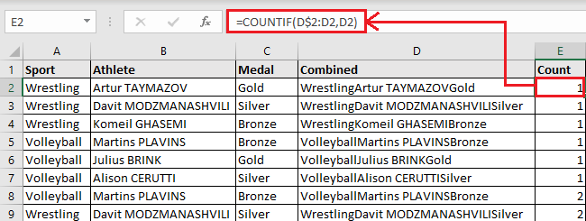
- Now, we will need another column named ‘Count to find out the duplicates in Column D. Hence, we use the COUNTIF function on cell E2. The formula will be:
=COUNTIF($D$2:D2,D2)
This formula helps count the number of occurrences of each value in column D.
-
If the Count value is “1”, the entry is unique. If the Count value is “2” or more, it indicates a duplicate.
Steps to Filter and Remove Duplicates:
- Check the Count:
- After using the
COUNTIFformula in column E, any cell with a value of “1” is unique, while any cell with a value of “2” or more is a duplicate.
- After using the
- Add a Filter:
- To filter out the duplicates, go to the DATA tab.
- In the Sort & Filter section, select Filter.
Path: DATA tab → Sort & Filter section → Filter
- Filter for Unique Values:
- Click on the filter arrow at the top of Column E (where you have the count of occurrences).
- Select the value “1” to filter out the rows that contain only unique values.
- Remove Duplicates:
- After filtering, only the rows with a Count value of “1” will be displayed, leaving out the duplicates.
- You can now copy these unique records and paste them into another location if needed.
By following these steps, you can effectively remove duplicate entries from your dataset, leaving only the unique records.

- Check the Count:
Let’s proceed by understanding the final approach to delete duplicates: Using Power Query.
